Gif showing a blue card on a green background. The card has a picture of a villager from Nintendo's Animal Crossing game with their name, personality type, species and hobby. A mouse cursor swipes the card to the right, meaning 'like', and another card appears with a different character. The card is swiped to the left, meaning 'dislike'.

tl;dr

I once wrote an R Shiny app to run a popularity contest for Animal Crossing villagers. Surprise: cute ones are favourites.

Swiping {shinyswipe} code

A while back I wrote a Shiny app (site, source, blogpost) for TidyTuesday to replicate a Tinder-like experience using villagers from Nintendo’s Animal Crossing New Horizons game. It uses the swipe mechanic from Nick Strayer’s {shinysense} package to gauge popularity: left for a ‘dislike’, right for a ‘like’.

After exceeding 3000 total swipes, it’s time to take a look at the results.

Oh sheet

Data from each swipe in the app is automatically appended to a public Google Sheets sheet that can be read with {googlesheets4}. Public sheets don’t require authentication to download, so run gs4_deauth() before read_sheet() to prevent it.

library(googlesheets4)
gs4_deauth()

raw <- read_sheet(
  ss = "1kMbmav6XvYqnTO202deyZQh37JeWtTK4ThIXdxGmEbs",
  col_types = "Tcc"  # datetime, char, char
)

## ✓ Reading from "acnh-swipe_results".

## ✓ Range 'Sheet1'.

First thing is to isolate the left and right swipes only. The {shinysense} package also allows for up and down swipes by default and I wasn’t sure how to remove this capability from my app (i.e. work lazier, not harder).

dat <- raw[raw$swipe %in% c("left", "right"), ]
dat[sample(rownames(dat), 5), ]  # random sample

## # A tibble: 5 × 3
##   date                name    swipe
##   <dttm>              <chr>   <chr>
## 1 2021-01-31 22:48:29 Renée   right
## 2 2020-11-09 02:16:26 Kid Cat right
## 3 2022-01-08 05:27:15 Agent S right
## 4 2020-09-29 04:18:40 Cleo    right
## 5 2020-09-15 07:25:45 Goose   left

The data are one row per swipe, with columns for date (datetime of when the swipe happened), name (the villager’s name) and swipe (the swipe direction).

But what we’re really after is a grouped table with a row per villager, plus new columns for the total number of swipes, the difference between right and left swipes and the percentage of swipes that were to the right (pc_right). These will let us better rank the characters.

df <- with(dat, table(name, swipe)) |>  # like dplyr::count()
  as.data.frame(responseName = "n") |>
  reshape(  # like tidyr::pivot_*()
    v.names   = "n",      # values_from
    idvar     = "name",   # id_cols
    timevar   = "swipe",  # names_from
    direction = "wide",   # i.e. pivot_wider()
    sep       = "_"       # names_sep
  ) |> 
  transform(  # like dplyr::mutate()
    total    = n_left + n_right,
    diff     = n_right - n_left,
    pc_right = 100 * round(n_right / (n_right + n_left), 2)
  )

head(df)

##      name n_left n_right total diff pc_right
## 1 Admiral      5       4     9   -1       44
## 2 Agent S      6       3     9   -3       33
## 3   Agnes      4       5     9    1       56
## 4      Al      6       3     9   -3       33
## 5 Alfonso      5       5    10    0       50
## 6   Alice      3       7    10    4       70

I think most readers of this blog are probably {tidyverse} users, so I’ll explain some of the base R approach I took here:

I’ve used the base pipe (|>) introduced in R v4.1 to chain the functions, which is analogous to {magrittr}’s pipe (%>%) in this example
with() allows the bare column names in table() to be evaluated as columns of dat, which means you only write the name of the data object once
a table() coerced with as.data.frame() is equivalent to dplyr::count(), basically
reshape() can be used like tidyr::pivot_wider() (I’ve added comments in the code block above to show how the arguments are used)
turns out that transform() can be used like dplyr::mutate() to create new columns, thought the help files say it should only be used for interactive and that ‘you deserve whatever you get!’

We can also bring in some additional villager data collected for TidyTuesday and join it to the swipe data. This will come in useful later.

tt <- read.csv(
  paste0(
    "https://raw.githubusercontent.com/rfordatascience/tidytuesday/",
    "2e9bd5a67e09b14d01f616b00f7f7e0931515d24/data/",
    "2020/2020-05-05/villagers.csv"
  )
)

df <- merge(df, tt, by = "name")

New Horizons scanning

There are 391 villagers represented in these data, with a combined total of 3234 legitimate swipes.

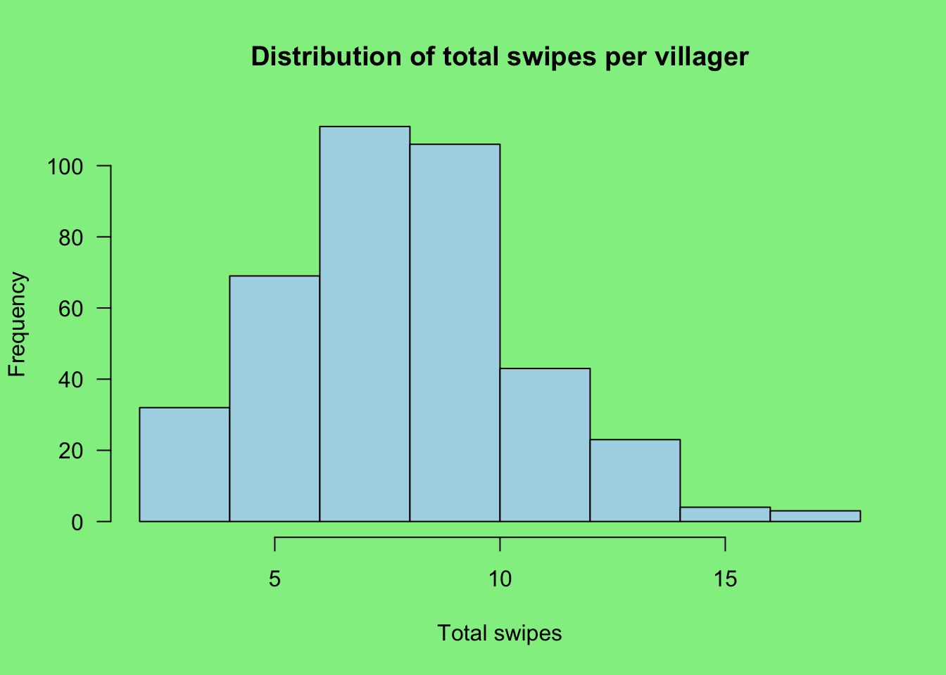
The total swipes per villager ranged from 2 to 17, with a mean of 8.3±2.7, so some characters didn’t really get enough swipes for proper assessment. You’d better go to the app and add some more swipes, eh?

par(bg = "lightgreen")
hist(
  df$total,
  main = "Distribution of total swipes per villager",
  xlab = "Total swipes",
  col = "lightblue",
  las = 1
)

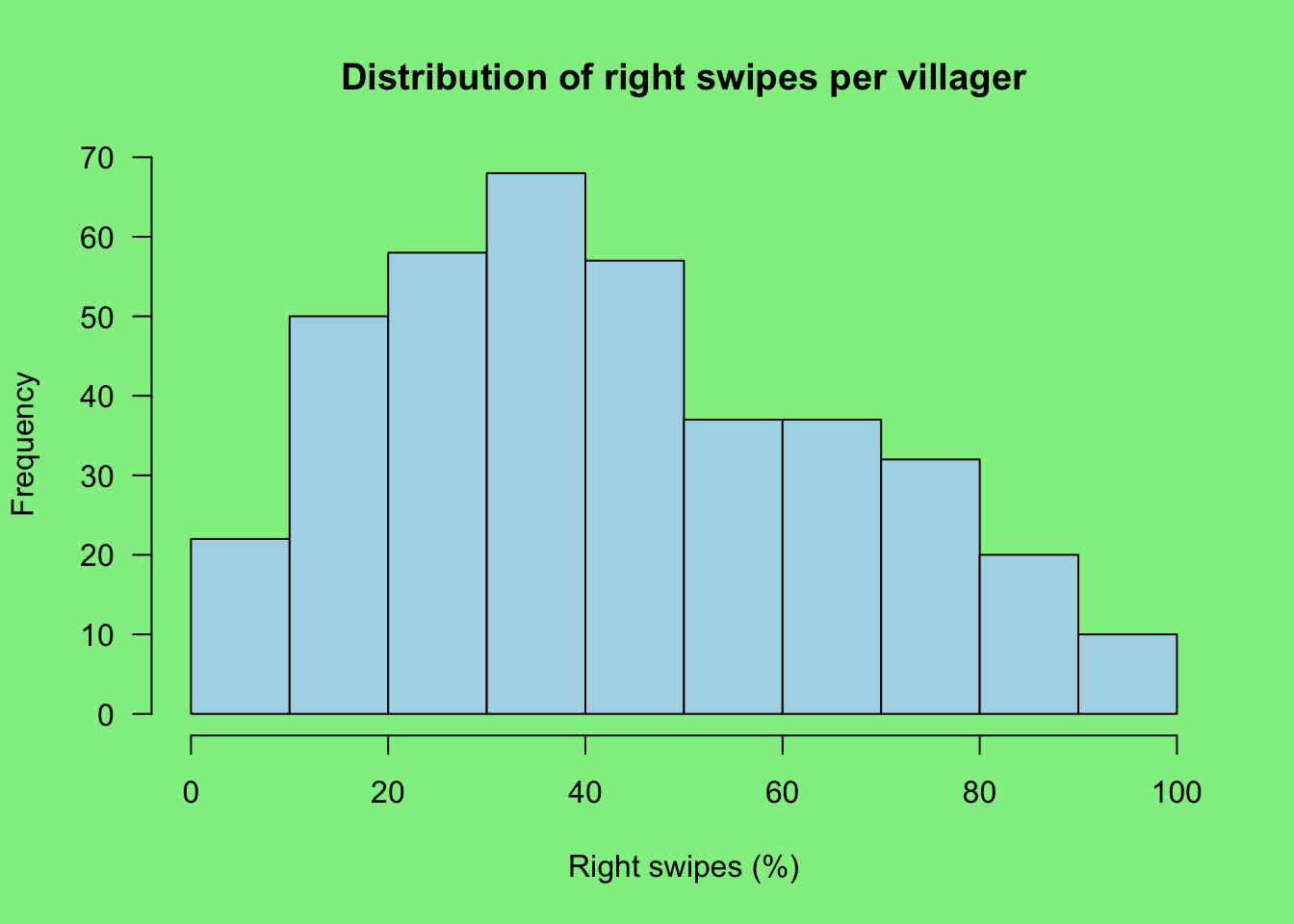
Histogram of total swipes per villager. It's roughly normally distributed between 5 and 10 swipes, but slightly left-skewed with a tail going beyond 15 swipes.

What if we look now at right swipes (i.e. ‘likes’), adjusted for the total swipes per character?

par(bg = "lightgreen")
hist(
  df$pc_right,
  main = "Distribution of right swipes per villager",
  xlab = "Right swipes (%)",
  col = "lightblue",
  las = 1
)

Histogram of the percentage of right swipes (likes) per villager. Nearly normal, with a slight skew to the left.

You can see that the distribution isn’t quite normal. The frequency of swipes below 50% is 227 and above 50% is 136. This implies that the majority of characters were disliked in a binary sense.

The bins at 0 and 100% tell you that there were some characters that were met with universal disapproval and approval, while the bin at 50% tells us that same characters split people’s opinions. Which were they?

Drumroll, please

So, onto the villager rankings.

I’ve written a little function to output an HTML table where each character’s name links to their profile on the Animal Crossing Wiki and exposes their photo from VillagerDB.

entable <- function(df) {
  df$url <- paste0(
    "<img src='", df$url, "' ",
    "width=50 ",
    "alt='Animal Crossing villager ", df$name,"'>"
  )
  df$name <- paste0(
    "<a href='https://animalcrossing.fandom.com/wiki/",
    df$name, "'>", df$name, "</a>"
  )
  df <- df[, c("name", "url", "pc_right", "total")]
  names(df) <- c("Name", "Picture", "Right swipes (%)", "Total swipes")
  rownames(df) <- NULL
  knitr::kable(df)
}

Least popular

To build tension, we’ll start with the least-liked villagers.

bot <- df[order(df$pc_right, -df$n_left), ] |> head()
entable(bot)

Name	Picture	Right swipes (%)	Total swipes
Pinky		0	12
Cashmere		0	9
Greta		0	9
Harry		0	9
Curly		0	8
Benedict		0	7

Sorry Pinky. You are simply… too pink? Seems harsh.

Most polarising

To build even more tension, let’s look at the characters who had a 50:50 ratio of likes to dislikes.

meh <- subset(df[order(-df$total), ], diff == 0) |> head()
entable(meh)

Name	Right swipes (%)	Total swipes
Chevre	50	14
Julian	50	12
Static	50	12
Vivian	50	12
Alfonso	50	10
Blaire	50	10

I’m not sure why these villagers are so controversial Perhaps they’re too ‘plain’ for some people? But Julian is a unicorn! With a sick space-themed hoody!

Most popular

And finally, what you’ve all been waiting for.

top <- df[order(-df$pc_right, -df$n_right), ] |> head()
entable(top)

Name	Right swipes (%)	Total swipes
Bea	100	9
Bill	100	9
June	100	8
Ellie	100	7
Aurora	100	4
Eugene	100	4

So! Bea and Bill were unanimously approved with nine right swipes each. I think the key trait here is ‘cuteness’: the favourites are generally small, big-eyed villagers (and Eugene’s Terminator aesthetic is charming on a koala).

Although Bill is staring directly into my soul.

Speciesism!

I know what you’re thinking: the results are on a villager-by-villager basis, but which species are the most popular? We can aggregate swipes and take a look.

sp_l <- aggregate(n_left ~ species, sum, data = df)
sp_r <- aggregate(n_right ~ species, sum, data = df)
sp_n <- with(df, table(species)) |> 
  as.data.frame(responseName = "n_villagers")

sp <- sp_n |> 
  merge(sp_l, by = "species") |> 
  merge(sp_r, by = "species") |> 
  transform(
    total = n_right + n_left,
    pc_right = 100 * round(n_right / (n_right + n_left), 2)
  )

A couple more base functions here for those not used to them:

aggregate() is like dplyr::group_by() followed by dplyr::summarise() and it allows for compact ‘formula syntax’, so we can say ‘aggregate y by x’ with y ~ x
merge() is just like the dplyr::*_join() family

So, firstly, the species ranked by lowest proportion of right swipes.

sp_bot <- sp[order(sp$pc_right, -sp$n_left), ]
rownames(sp_bot) <- NULL
head(sp_bot)

##   species n_villagers n_left n_right total pc_right
## 1   mouse          15     90      19   109       17
## 2   eagle           9     54      17    71       24
## 3   hippo           7     43      15    58       26
## 4    bull           6     40      14    54       26
## 5    bear          15     87      32   119       27
## 6 chicken           9     49      20    69       29

I can see how eagles, monkeys and hippos might not be that ‘cute’, per se, but what about the mice? Although ‘cute’ is probably not the best term for the cranky mouse Limberg (sorry Limberg).

What about the most liked species?

sp_top <- sp[order(-sp$pc_right, sp$n_right), ]
rownames(sp_top) <- NULL
head(sp_top)

##   species n_villagers n_left n_right total pc_right
## 1 octopus           3      6      18    24       75
## 2   koala           9     17      43    60       72
## 3     cub          16     43      74   117       63
## 4     dog          16     49      80   129       62
## 5    deer          10     43      67   110       61
## 6    wolf          11     33      50    83       60

Octopuses are on top, although there’s relatively few octopus villagers. Personally, I like Zucker, an octopus who looks like takoyaki and therefore delicious.

This wasn’t meant to be about villager tastiness, was it? We may need a new app to rank by apparent edibility…

The most popular Animal Crossing villagers